 Embryo series courtesy of Einhard Schierenberg
Table of Contents
In C. elegans, the expression pattern of a gene provides important clues to understanding its biological function. To accurately depict endogenous transcriptional activity, a highly sensitive method is required to measure transcript levels in the intact tissue across various developmental stages. Conventional RNA in situ hybridization methods using hapten- (biotin or digoxygenin) labeled RNA probes rely on antibody binding for visualization, and are thus only semi-quantitative at best (Raap et al. 1995; Levsky et al. 2003). Additionally, hapten-labeled probes are prone to diffuse localization (when conjugated with alkaline phosphatase), low sensitivity (when conjugated with fluorescent molecules), and non-specific probe binding. Here, we introduce a recently developed mRNA in situ hybridization method (Raj et al. 2008) that circumvents the above difficulties to give single molecule resolution of transcript detection.
The single molecule fluorescent in situ hybridization (smFISH) method differs from conventional approaches by using many short (about 20 base pairs long) oligonucleotide probes to target different regions of the same mRNA transcript (Raj et al. 2008; Femino et al. 1998). Each oligo is conjugated with only one fluorophore and thus faintly visible by itself. Binding of multiple oligos to the same transcript yields a bright spot, indicative of a single mRNA transcript. Since mis-bound probes are unlikely to co-localize, this method effectively reduces false-positive signal from non-specific probe binding. The small oligo size allows the probes to efficiently penetrate through target tissue, yielding robust detection of even low-abundant transcripts. Subsequently, the total number of fluorescent spots within a single cell or region can be unambiguously counted and compared across different developmental stages and genetic backgrounds.
Given its many advantages, the smFISH method is a powerful tool to study transcriptional regulation. Its high sensitivity allows accurate characterization of the spatio-temporal patterns of endogenous gene expression. Its single-molecule resolution enables precise quantification of gene expression levels. Such quantitative information can in turn be used to assess, for example: 1) tissue-specific correlations in gene expression, 2) similarity and difference in gene expression across strains, 3) variability in gene expression, and 4) tissue-specific signaling dynamics. To date, smFISH has been successfully applied to study a variety of questions in C. elegans biology (Raj et al. 2010; Harterink et al. 2011; Korzelius et al. 2011; Middelkoop et al. 2012; Saffer et al. 2011; Seidel et al. 2011; Topalidou et al. 2011). Here we provide the necessary technical details to set up and perform smFISH, from sample preparation to data analysis.
The following protocol covers the 5 major steps of smFISH: A. Probe design and synthesis, B. Fixation of C. elegans worms and embryos, C. Hybridization, D. Image acquisition, E. Data analysis. This protocol is largely adapted from the general smFISH protocol detailed in Raj and Tyagi (2010), with notes and modifications specific to C. elegans. Unless otherwise noted, all reagents listed can be made in bulk ahead of time and stored at room temperature (RT).
smFISH probes are DNA oligonucleotide probes designed according to the follow criteria:
Probe length: 17-22 base pairs
Probe spacing: no less than 2 base pairs
Probe GC content: ideally around 45% to ensure uniform binding efficiency
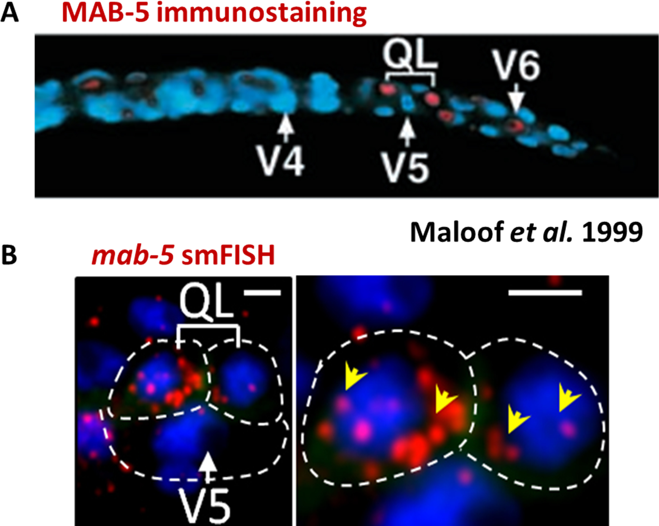
Number of probes: ideally between 30 and 96 depending on target transcript length. Typically 48 probes are used to ensure good signal quality, while as few as 20 have yielded satisfactory signal (e.g., Figure 1 illustrates the result from 27 probes designed to target mab-5 mRNA). To increase effective target length, part or all of the 3’UTR sequences can be combined with the cDNA sequence for probe design.
|
Figure 1. Comparison of immunohistochemistry and smFISH results detecting mab-5 expression in the QL neuroblasts. A. MAB-5 immunostaining of a wild-type L1 larva. MAB-5 expression is seen in the two QL daughters above V5. (Adapted from Maloof et al. 1999) B. mab-5 mRNA detected by smFISH in L1 larva around the same age. Note the asymmetry in mab-5 mRNA abundance between the two QL daughters. Scale bars are 2.5 μm.
A web-based probe design software developed by Raj et al. (2008) is available free of charge at: http://www.biosearchtech.com/stellarisdesigner/. By supplying the target RNA sequence and the above criteria, one obtains a list of probe sequences with optimized GC contents. These sequences can then be directly submitted for probe synthesis.
Synthesis: Based on the designed oligonucleotide sequences, smFISH probes are generated en masse using a 96-well DNA synthesizer. Biosearch Technologies (Novato, CA) offers synthesizing service for custom-designed smFISH probes. The probes can be ordered in both coupled and uncoupled forms. While ordering coupled probes minimizes the work involved in probe preparation, obtaining uncoupled probes allows the flexibility to choose fluorophores that are optimally compatible with the researcher's microscope setup (e.g., filter cubes) and other experimental needs. Furthermore, coupled probes are delivered as a mix, which precludes the option of using subsets of the probe library to 1) selectively target different parts of the transcript, or 2) perform negative controls using deletion mutants (see additional comment in the following section and details of suggested controls in the Controls and Troubleshooting section). In the following section, we further suggest a list of factors to consider when deciding whether to pursue in-house coupling.
Given the small amount of probes needed for each hybridization experiment, synthesis can be carried out at a small scale (Biosearch now delivers 5 nmol of each probe per custom order. This amount is typically sufficient for hundreds of experiments). When ordering uncoupled probes, the oligonucleotide probes should be synthesized with a 3’amine group to allow subsequent oligo-fluorophore conjugation. Additionally the oligos should be desalted and resuspended in water as opposed to Tris EDTA (TE), which can interfere with subsequent amine-coupling reactions.
Coupling:
Note: When deciding whether to perform in-house coupling or order readily coupled probes, we suggest considering the following:
Is it clear which fluorophore to choose? This could vary depending on probe set and the optical setup.
Is it necessary to split the probe sets to target different parts of a transcript? Pre-coupling requires mixing of all probes in a library, thus excluding the possibility of alternative probe combinations.
Is in-house coupling feasible? Is there access to a nearby HPLC facility?
Does experimental schedule allow an additional 3-4 days of probe preparation?
Is budget a concern? A single probe set of 10 nmol quantity can be coupled to multiple fluorophores (up to 3-4 coupling per probe set is possible), avoiding the need to purchase multiple libraries.
Prior to coupling, one needs to decide on the desired type of fluorophore. The current protocol uses succinimidyl ester derivatives to couple to the 3’ end of the oligonucleotide probes. Three types of commercially available fluorophores are commonly used: Cy5 (GE Amersham), Alexa 594 (Molecular Probes, Invitrogen), and tetramethylrhodamine (TMR) (Molecular Probes, Invitrogen). Biosearch also offers equivalent fluorophores (Quasar 670, and CAL Fluor 610 and 590) for their couple probe sets. In general we have found that using fluorophores with shorter emission wavelengths (such as Alexa 488) does not yield reliable signal due to high cellular autofluorescence. Table 1 summarizes the strengths and weaknesses of each of the fluorophores as observed in our hands.
Table 1. Strengths and weaknesses of fluorophores commonly used in smFISH.
| Peak Excitation/Emission Wavelength | Photostability | Autofluorescence level | RFP compatible | GFP compatible | |
|---|---|---|---|---|---|
| Cy5 | 649/670 nm | Low | Low | Yes | Yes |
| Alexa 594 | 590/617 nm | High | Medium | Affected | Yes |
| TMR | 564/570 nm | High | High | No | Yes |
For multiplexing assays, we have obtained good results with combinations of all three dyes (provided that each probe set works well when assayed on its own). We generally prefer to pair Cy5 with Alexa 594, as the two fluorophores tend to give better signal quality than TMR. For initial testing, it is important to compare results from multiplex and single-fluorophore assays to ensure consistency. Also keep an eye out for “suspiciously similar” spot patterns accross channels, which is indicative of cross-talk between fluorescent channels.
Reagents for coupling:
DMSO (if coupling to TMR)
*0.1 M Sodium Bicarbonate (in RNase free water, pH 8.0)
*1 M Sodium Bicarbonate (in RNase free water, pH 8.0)
Ethanol (>95% pure)
3 M Sodium Acetate, pH 5.2
Fluorophore with succinimidyl ester group
*Note: it is desirable to make sodium bicarbonate fresh, or check before use to make sure the pH level is correct.
Day 1:
From the uncoupled probe stock, combine 1 nmol (e.g., 10 μl from a 100 μM stock) of each probe into a single microcentrifuge tube.
Add 0.11 volumes 1 M sodium bicarbonate to give a final concentration of 0.1 M. If the total volume at this stage is < 0.3 mL, add some 0.1 M sodium bicarbonate to bring total volume to 0.3 mL.
Dissolve a small amount (roughly 0.2 mg) of dye into 50 μl of 0.1 M sodium bicarbonate.
Note: TMR can be hard to dissolve in aqueous solution, so one must first dissolve it in a small volume (<5 μl) of DMSO before adding 50 μl of 0.1 M sodium bicarbonate.
Add the dissolved fluorophore to the oligos.
Cover the tube in foil to prevent photo-bleaching and let the reaction proceed overnight at room temperature with gentle rocking.
Day 2:
In the morning, precipitate the oligos by adding 10% volume/volume of 3M sodium acetate and then adding 2.5 volumes of 100% EtOH. Store at −70°C for at least 1 hour (up to overnight).
Spin down the sample in a 4°C microcentrifuge for at least 15 minutes at maximum speed (~16K RCF).
After centrifugation, one should see a small colored pellet at the bottom of the tube. Aspirate away the fluorescent supernatant (containing uncoupled dye molecules) as completely as possible. If purification is not performed right away, the pellet is stable and can be stored at −20°C.
Purification: The pellet obtained from the coupling steps contains a mixture of coupled and uncoupled oligonucleotides. To separate the two species, we take advantage of the fact that coupled probes experience a large increase in hydrophobicity compared to the uncoupled ones. High-pressure liquid chromatography (HPLC) can thus be used to enrich for coupled probes.
Reagents and equipments for purification:
0.1 M Triethylammonium acetate, pH 6.5, filtered and degassed (Buffer A)
Acetonitrile for HPLC (Buffer B)
HPLC with a dual wavelength detector to measure both DNA and fluorophore absorbtion
C18 Column for HPLC, 218TP104
SpeedVac rated for acetonitrile
Day 2 (if continued immediately after coupling step 8):
Resuspend pellet in appropriate volume (0.1→0.5 mL nuclease free water, depending on your HPLC)
Inject coupled probe into HPLC and run a program in which the percentage of buffer B varies from 7% to 30% over the course of around 30 minutes with a flow rate of 1 mL/minute.
Note: Set the detector to monitor DNA absorption (260 nm) and the absorption of the coupled fluorophore (e.g., 555 nm for TMR).
One will observe two broad peaks. The first contains uncoupled probes and will only show a peak in the 260 nm channel. The second contains pure coupled probes and will show peaks in both channels. The two peaks will typically be separated by a few minutes of time or longer, with TMR having narrowly separated peaks and Cy5 having broadly separated peaks. With a series of microcentrifuge tubes, collect the entire second peak as soon as the signal begins rise and until it drops back to baseline.
Day 3:
Dry the purified probes in a SpeedVac vacuum concentrator (~ 3-5 hours for 0.5 mL).
Note: Be sure to prevent any light from hitting the probes during the drying process to prevent photobleaching, especially for photolabile dyes such as Cy5.
Resuspend all tubes together in a total of 50-100 μl of TE, pH 8.0 (equivalent to roughly 0.1–1 μM). This is the concentrated probe stock.
(Optional) Dilute this probe 1:10, 1:20, 1:50 and 1:100 in TE to make working stocks for testing probe concentration.
At this point, probe synthesis is complete. Probes can be stored in TE at −20°C for years.
Reagents for fixation:
Fixation solution: 4% paraformaldehyde (PFA) in 1x PBS
Bleaching solution for embryos (per 40 mL, store at 4°C):
40 mL distilled water
7.2 mL 5 N NaOH
4.5 mL 6% NaHOCl
M9 buffer (per 1L):
5.8 g Na2HPO4
3.0 g KH2PO4
0.5 g NaCl
1.0 g NH4Cl
Dissolve in distilled water (dH2O) to 1 L final volume
Fixation protocol for worms (larvae and adult):
Grow worms on plates seeded with OP50. Synchronize worms to the desired stage if needed.
Note: The appropriate number of plates may vary depending on need, with the minimum requirements that 1) there will be enough worms to form a visible pellet in a microcentrifuge tube, and 2) each plate is not too crowded.
Add 3-5 mL M9 buffer to the plate and swirl to release worms from surface, then transfer worms to a 15 mL conical centrifuge tube.
Note: Distilled or deionized water may be used instead of M9 in this and subsequent steps.
Spin down to form a pellet and aspirate the supernatant.
Wash and spin down with 3-5 mL M9 buffer to rinse away bacteria and other debris.
Resuspend in 1 mL fixation solution and transfer to microcentrifuge tube. Keep rotating at room temperature for 45 min.
Note: Since autofluorescence levels increase with fixation time, incubation in fixation solution should be kept short. This is especially important for older worms where tissue autofluorescence is relatively strong.
Wash twice with 1 mL 1x PBS.
Resuspend in 1 mL of 70% EtOH. Keep rotating for overnight (or longer) at 4°C. Store at 4°C for up to a month.
Fixation protocol for embryos:
Grow worms on OP50 plates till there are plenty of gravid hermaphrodites.
Wash worms off the plates with M9 into a 15 mL conical centrifuge tube.
Note: Distilled or deionized water may be used instead of M9 in this and subsequent steps.
Spin down and resuspend in bleaching solution. Vortex or shake rigorously for 4-8 minutes until worms disappear and only embryos remain.
Spin down and aspirate. Then wash twice with M9 buffer.
Resuspend in 1 mL fixation solution and transfer to a microcentrifuge tube. Keep rotating at room temperature for 15 minutes.
Vortex and then immediately submerge tube in liquid nitrogen for 1 minute to freeze crack the eggshells.
Thaw in water at room temperature.
Once thawed, vortex and place on ice for 20 minutes.
Wash twice with 1 mL of 1x PBS.
Resuspend in 1 mL of 70% EtOH and keep rotating for overnight or longer at 4°C. Embryos can be hybridized up to a week following fixation.
Reagents for hybridization:
Hybridization buffer (per 10 mL, store at −20°C freezer):
*1 g dextran sulfate
10 mg Escherichia coli tRNA
100 μl 200 mM vanadyl ribonucleoside complex (New England Biolabs, Inc.)
40 μl 50 mg/mL RNase free BSA (Ambion)
**Formamide (deionized, Ambion)
Add nuclease free (NF) water (Ambion) to 10 mL final volume
* Note: Dextran sulfate is viscous and hard to dissolve at room temperature. One solution is to mix dextran sulfate with 4 mL NF water, then sonicate till no clumps are visible.
** Note: Determine the amount based on the desired formamide concentration, e.g., 1 mL for 10% final concentration. Higher concentration yields higher probe binding stringency.
Wash buffer (per 50 mL):
Formamide (deionized, Ambion), use same concentration as determined for hybridization buffer
5 mL 20x SSC (RNase free, Ambion)
Add NF water (Ambion) to 50 mL final volume
DAPI stain: Prepare working stock of 5 ng/mL in RNase free water, store in the freezer.
2x SSC: Prepare from 20x SSC (RNase free, Ambion) in RNase free water (Ambion).
Antifade buffer (to be made fresh)
Glox buffer (per 50 mL):
2 mL 10% glucose in NF water
250 μl 2M Tris-HCl, pH 8.0
5 mL 20x SSC (RNase free, Ambion)
Glycosidase stock: Dilute commercial Glox (glucose oxidase, Sigma-Aldrich) in 50 mM sodium acetate to working stock of 3.7 mg/mL, adjust to pH 5.0. Aliquot to 100 μl units and store at −20°C.
Catalase (Sigma-Aldrich): store at 4°C.
Prior to imaging, mix 1 μl each of the glycosidase stock and catalase into 100 μl of Glox buffer. Each 100 μl antifade mix is enough for 1–2 hybridization samples.
Day 1:
Prepare the hybridization solution: to 100 μl of hybridization buffer, add 1 μl of each probe at the appropriate concentration, then vortex and centrifuge.
Note: For the initial test of probe concentration, one may perform four parallel hybridizations with probes diluted at 1:10, 1:20, 1:50 and 1:100 in TE. In our hands, 1:20 works well for Cy5 coupled probes and 1:50 appears sufficient for Alexa 594 coupled probes.
Centrifuge the fixed sample and aspirate away the ethanol.
Resuspend in 1 mL wash buffer that contains the same concentration of formamide as the hybridization buffer. Let stand for 2–5 min.
Centrifuge sample and aspirate away the wash buffer.
Add the hybridization solution prepared in step 1. Incubate overnight at 30°C in the dark.
Note: The modified protocol on the Biosearch website now recommends 4 hour incubation at 37°C. We plan to try out this modification and compare the results carefully with our existing data sets. The result will be included in a future edition of this protocol.
Day 2:
In the morning, add 1 mL wash buffer to the sample. Vortex, spin down and aspirate.
Resuspend in another 1 mL wash buffer and incubate at 30°C for 30 min.
Spin down and aspirate. Resuspend in 1 mL wash buffer
Add 1.5 μl DAPI stain (5 ng/mL) for nuclear counterstaining. Vortex and incubate at 30°C for 30 min.
Spin down and aspirate the wash buffer. Resuspend in 2x SSC, vortex, spin down and aspirate.
If imaging without glox antifade solution (possible for Alexa 594 and TMR), resuspend in a small amount (enough the cover the samples) of 2x SSC and proceed to imaging.
If imaging with the antifade solution, resuspend in a small amount of glox buffer and proceed to imaging.
Note: While hybridized samples can be stored temporarily in 2x SSC at 4°C. Prolonged storage increases the risk of signal degradation. It is thus advisable to image immediately following hybridization.
Note: The hybridization protocol posted by Biosearch (http://www.biosearchtech.com/assets/bti_custom_stellaris_celegans_protocol.pdf) differs from ours in the following: 1) omission of the blocking reagents (tRNA and BSA) from the hybridization buffer; 2) hybridize at 37°C (instead of 30°C) for 4 hours (instead of overnight). At the moment, we have not tried or systematically compared their protocol with our results. We plan to do so and will report our results in a future edition of this protocol.
Microscopy equipment:
Microscope: Standard wide-field fluorescence microscope (e.g., Nikon TE2000 or Ti, Zeiss Axiovert).
Note: Confocal microscopes, while excellent in spatial precision, use high light intensity and cause rapid bleaching of smFISH signals. They are especially problematic when taking multiple z sections and are thus not recommended for smFISH imaging.
Light source: A strong light source is essential for spot detection. Mercury or metal-halide lamp (e.g., ExFo Excite, Prior Lumen 200) are both good candidates. The metal-halide lamps are generally brighter and thus ideally suited for far-red dyes such as Cy5.
Note: With a metal-halide lamp, the exposure time we use for smFISH signal detection is generally around 1-2s, while only 100–200 ms is needed for GFP and DAPI.
Filter sets: Three filters, excitation, dichroic, and emission filters, are needed for each fluorescent channel. Choice of filters should be made based on the optical features of the corresponding fluorophores used (see Table 2 for a list of the filters we use).
Camera: Standard cooled CCD camera optimized for low-light level imaging rather than speed (preferably with 13 mm pixel size or less; e.g., CoolSNAP HQ from Pixis, Princeton Instruments).
High numerical aperture (NA> 1.3) 100x DIC objective (be sure to check transmission properties when using far red dyes such as Cy5 or Cy5.5). We have also seen spots using an oil-immersion 60x objective, but the reduced spatial resolution makes the spots somewhat more difficult to identify computationally.
Table 2. Examples of optical filter sets compatible with multiplex mRNA detection
| Excitation | Dichroic | Emission | Supplier | |
|---|---|---|---|---|
| Cy5 | HQ620/60x | Q660LP | HQ700/75m | Chroma |
| Alexa 594 | 590DF10 | 610DRLP | 620DF30 | Omega |
| TMR | 546DF10 | 555DRLP | 580DF30 | Omega |
Software: Standard microscopy software capable of memorizing sample positions and imaging through z optical stacks. We currently use MetaMorph (Molecular Devices), which offers easily programmable user interface.
Imaging chamber: There are two purposes of the imaging chamber: 1) to affix the sample in a small region and prevent drying and 2) to minimize the thickness of the sample by flattening, thereby reducing out of focus light. To assemble the chamber:
Pipette 2-5 μl of the sample in antifade solution onto a clean 8mm round cover glass (Electron Microscopy Sciences, #1.5 thickness).
Gently tap a clean 22 × 22 mm square cover glass (VWR, #1 thickness) onto the drop of sample solution. This will cause the round cover glass to quickly adhere to the square glass.
Optional: Clean cover glasses before hand by rinsing with 70% EtOH and let dry.
Immediately flip the square glass so that the round glass is on top. Let sit for half a minute or so while covered in dark.
While waiting, adhere a square Silicone Isolator (Grace Biolabs, 20 mm diameter × 0.5 depth) to a regular microscope slide.
Gently remove excess antifade solution from the rim of the round cover glass with a Kimwipes wiper.
Adhere the square cover glass to the Silicone Isolator with the round cover glass facing towards the microscope slide. Press down on the edges of the square glass to create a tight seal. This constitutes the imaging chamber.
Affix the imaging chamber to the microscope stage. Make sure to position the microscope slide correctly so that the imaging chamber faces the objective. Proceed to locate individual worms or embryos.
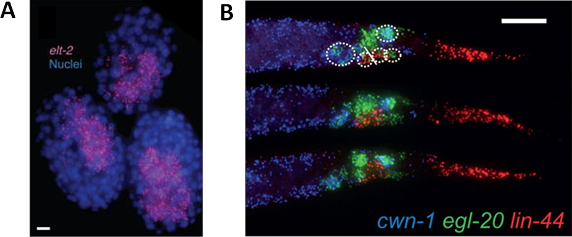
What to expect: A successful hybridization and sample preparation should yield clear fluorescent spots roughly 200-500 nm in size. These spots are so called “diffraction limited spots” based on the fact that the size of an mRNA molecule (nm) is far below the optical limit of the widefield microscope (μm). On a digitally acquired smFISH image, spot intensities usually vary within 2 fold of one another (for the same gene detected in the same fluorescent channel), with the exception of transcription centers in the nuclei (where large amounts of nascent transcripts accumulate), which can be much brighter. Optimal smFISH signal should be more than 1.5 times in intensity above the tissue background. When viewed on an image, the spots should be distinct in shape (i.e., not blurred) and readily identifiable by eye. Figure 2 illustrates two smFISH experiments, one probing elt-2 (a transcription factor involved in specifying the future intestine, Fukushige et al. 1998) in embryos (from Raj et al. 2010), the other staining three Wnt ligands expressed in the posterior body of the L1 larvae (from Harterink et al. 2011).
|
Figure 2. Examples of smFISH staining from embryos and L1 larvae. A. Detection of elt-2 mRNA (cyan spots) in mixed stage embryos. Scale bar is 5 μm long. (Adapted from Raj et al. 2010) B. Detection of three Wnt ligands, cwn-1, egl-20 and lin-44, in the posterior body of staged L1 larvae. Scale bar is 10 μm long. (Adapted from Harterink et al. 2011).
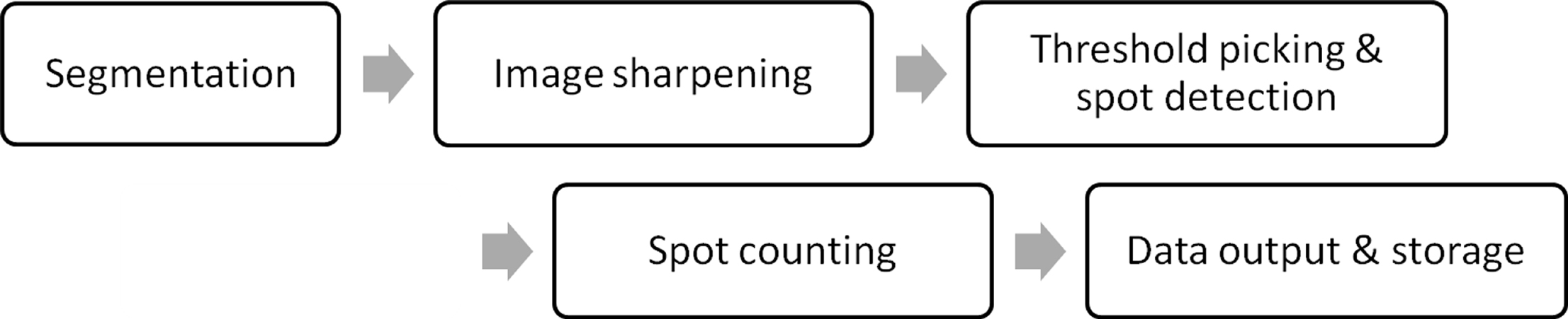
Successful smFISH experiments can simultaneously provide high quality information on the location, abundance, and transcriptional states of multiple mRNA species. To extract this wealth of information in an efficient and unbiased way, we recommend analyzing smFISH data using custom written computer software. While the exact analysis procedure may vary depending on experimental goals, we suggest the following analysis streamline (Figure 3) and briefly outline its implementation:
Image conversion: Common imaging softwares such as MetaMorph and NIH-image save images in .tiff or .stk format. These files are not directly analyzable in computing software such as MATLAB, and must be converted to a readable format.
*Note: A MATLAB code that reads data from .tiff files is available online at MATLAB Central: http://www.mathworks.com/matlabcentral/fileexchange/10298
Image segmentation: Image segmentation is a useful step in localizing mRNA expression to specific cell or tissue-types. Oftentimes, it is possible to take advantage of DAPI staining (for demarcating the body axes and major tissue groups, i.e., body wall muscles, ventral nerve cord, intestinal cells, etc.), GFP reporter systems, and smFISH signals (by staining for genes previously known to be expressed in a given cell or tissue) to accurately assign smFISH spots to their tissue of origin. Computational software can facilitate this process by overlaying images from multiple channels (e.g., Cy5, Alexa 594, GFP and DAPI), followed by manual or automatic annotation of the relevant spatial landmarks. These annotations can later be overlaid onto the smFISH images to allow tissue-specific transcript quantification. Additional analysis, such as measurement of tissue length or size, can also be performed computationally at this step. If performing segmentation using computational software (e.g., MATLAB), the resulting traces and annotations can be saved as a standalone data file and used for region-specific spot counting (step 5) later.
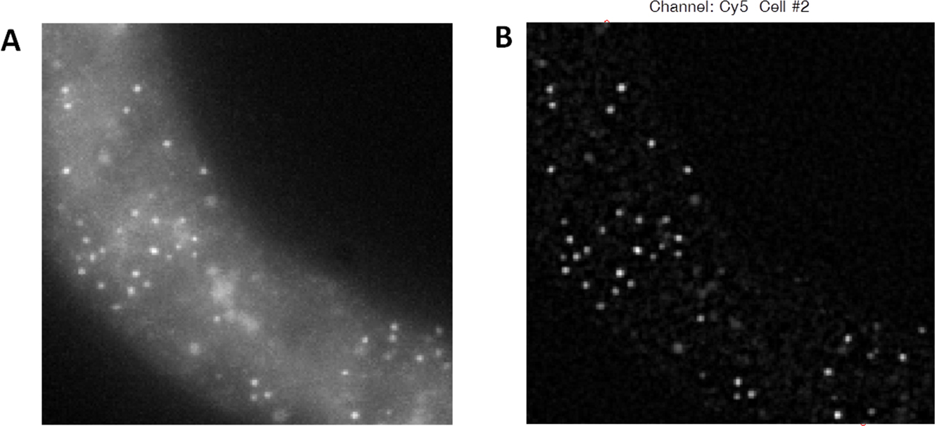
Image sharpening: To facilitate subsequent automatic spot detection, it is useful to first enhance the signal-to-noise contrast of the smFISH images. This can be done by convolving each image file (i.e., a matrix consisting of individual pixel values) with two mathematical functions (kernels), a Gaussian followed by a Laplacian. In practice the two functions can be convolved first to form a computational filter called the Laplacian of Gaussian (LoG). As shown in Figure 4, the effect of convolving the original image with the LoG filter is twofold: 1) the Gaussian filter smoothens the background to reduce small speckles that could be confused with real spots, 2) the Laplacian filter then performs edge detection by amplifying the contrast between adjacent dim and bright pixels. The width of the Gaussian filter should be picked to resemble the size of a typical spot. Alternatively, this can be done by trial and error (we recommend starting around 1.5) by visually comparing the filtered and original images. The following is an example of MATLAB code used for image sharpening:
H = -fspecial('log',15,1.2); % H is the LoG filter with a standard deviation of 1.2 and width around 5
g = imfilter(im,H); % im is the original smFISH image
Spot detection and semi-automated threshold picking: Since smFISH signals are significantly brighter than the background, individual spots are detected by identifying regions in the image with pixel values higher than a pre-specified threshold. One way of determining this threshold is to systematically screen threshold values in incremental steps from the minimum to the maximum pixel intensities. For each threshold value tested, the software identifies filled regions (or “connected objects”) wherein all pixel values are above threshold. The total number of filled regions is then summed up to yield the total spot count corresponding to the given threshold.
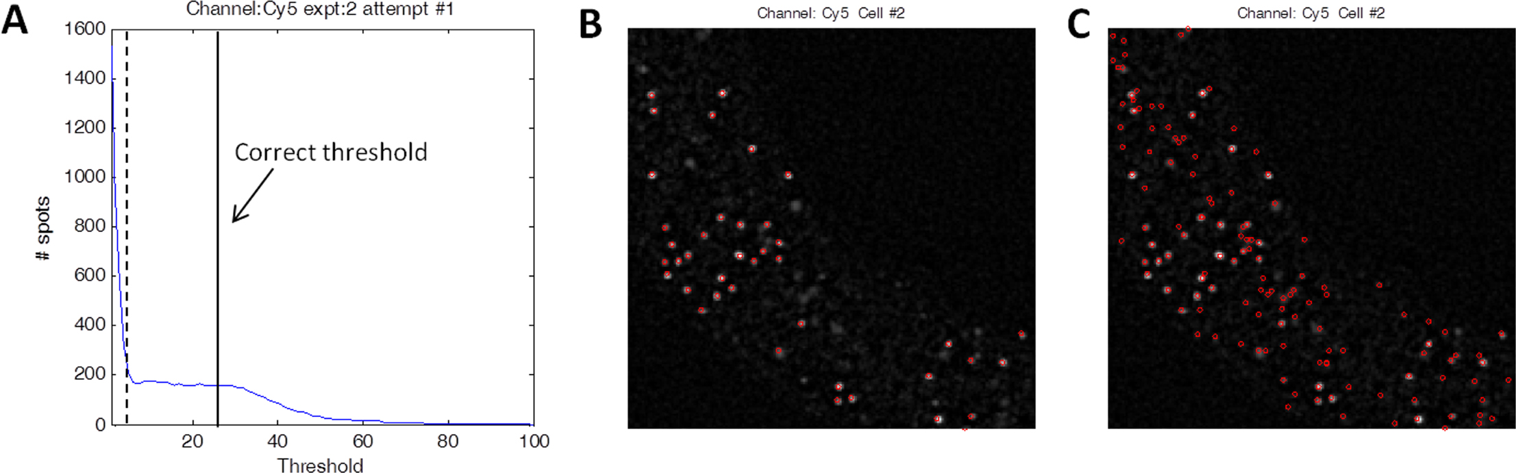
After spot detection and counting has been carried out for all thresholds, a plot can be generated showing total spot counts as a function of different threshold values. With high quality imaging data this curve is expected to start high and drop rapidly to reach a brief plateau, before it finally approaches zero (Figure 5). The observed plateau corresponds to all threshold values above the background auto-fluorescence and below the real signal intensity. The total spot count is approximately constant in this range and corresponds reliably to the number of actual smFISH spots. Seemingly convenient, automatic detection of this plateau is sometimes difficult (since the size and flatness of this plateau varies from image to image). Especially during initial testing of the software, we recommend to manually pick the threshold, and plot the computationally detected spots over the original image to ensure that no over- or under-counting has occurred.
Region-specific spot counting: Spot quantification within a specific cell or tissue can be conveniently achieved by aligning the results from image segmentation and spot detection. Computationally this can be done by generating a binary map for the region of interest (ROI) and using this map to filter out detected spots that are outside the ROI. MATLAB's Image Processing Toolbox provides many built-in functions that can greatly facilitate the image analysis steps described here. A sample of such MATLAB based software is available at the Arjun Raj lab website http://rajlab.seas.upenn.edu/pdfs/raj_nat_meth_2008_software.zip. Additional details for using MATLAB to perform image processing and single-molecule identification can be found in a recent paper by Scott Rifkin (2011). Other programming platforms, e.g., Python and Image J, also hold great promise in generating fast and accurate analysis software.
|
Figure 4. Effects of LoG filtering on smFISH images. A. Raw image data staining lin-17 mRNA in an L1 larva (shown is a single image from a stack). B. The same image after processing by a LoG filter with the above MATLAB commands. Note dramatic reduction in background and enhancement in spot signal.
|
Figure 5. Threshold picking and automatic detection of smFISH spots. A. Total spot counts as a function of pixel intensity threshold. The correct threshold should be placed where the spot count is insensitive to threshold value (where the “plateau” is). B. Spot detection when correct threshold (solid vertical line in A) is chosen. Red circles indicate computationally identified spots for a single image from a stack. Note out-of-focus spots are not counted. C. Spot detection when threshold is chosen too low (dotted line in A). Note many out-of-focus spots and background speckles are mistakenly included as spots.
As the power of smFISH method lies in the accurate detection of single mRNA molecules, it is important to perform proper controls for each new smFISH probe library generated. Here we outline a number of control experiments that address common concerns regarding smFISH results. Additionally, while the smFISH protocols described here worked robustly for many C. elegans genes (including Wnt and Notch pathway genes, endoderm specification genes, etc., in both worms and embryos), we did notice a number of technical factors that can affect data quality. We thus provide a list of troubleshooting tips below to facilitate further optimization of the protocols.
Recommended controls:
Does a single smFISH spot represent a single mRNA molecule?
Solution 1: To confirm single molecule resolution, one may randomly sample the peak pixel intensities of individual smFISH molecules within a given series of images (a process automatable by computer software). The spot intensities should then be plotted on a histogram. The resulting distribution is expected to be unimodal with one narrow peak (this would not be the case if mRNA molecules frequently occur as groups of two or more) (Vargas et al. 2005). Large mRNA aggregates in the nucleus or specialized organelles (as in the case of transcription centers, P bodies and stress granules) are often many-fold brighter and can be easily excluded from analysis by pixel thresholding. To control for the rare case where mRNA of the same species dimerize (an example being the Drosophila bicoid mRNA, Wagner et al. 2004), one may proceed to perform quantitative reverse-transcription PCR (qRT-PCR) as described below.
Solution 2: To independently check mRNA level, a control qRT-PCR experiment can be performed on bulk collected C. elegans tissue. As it is currently difficult to enrich for particular tissue or cell types in a bulk collection (with the exception of dissected gonads), this approach would only apply to whole worm or embryo measurement. qRT-PCR measurement from bulk collected tissue then needs to be normalized by the estimated total number of worms or embryos. The obtained average expression level per animal can then be compared to average smFISH measurements, and the two are expected to be largely consistent.
Are we robustly detecting all mRNA transcripts of a given species? (Positive control)
Solution 1: Separate the uncoupled probe library into two halves containing non-overlapping sets of probes. Couple these two probe sets respectively with two different fluorophores and hybridize both probe sets to the same sample. If the majority of mRNA transcripts are reliably detected, most spots should appear double labeled, and the overall degree of co-localization should be high. We have consistently detected around 85% co-localization, suggesting the majority of the mRNA transcripts are being detected by smFISH. Additionally, it is recommended to partition the probe library in a way that allows probes with one fluorophore to interleave probes with the other fluorophore. Compared with having the two sets of probes targeting two different regions of the endogenous mRNA, this approach avoids differences in probe binding efficiency along different parts of the mRNA. A potential weakness is that this approach is non-robust for mRNAs that are inaccessible by the smFISH protocol (e.g., mRNAs that are localized in specialized organelles or embodied by protein complexes). The following approach provides an independent and complementary assessment of total mRNA quantity.
Solution 2: To determine whether the number of transcripts detected by smFISH is accurate, one may perform, in parallel, quantitative reverse-transcription PCR (qRT-PCR) on a known number of synchronized worms. The total and average number of transcripts should agree between the two approaches. However this approach may not work well when transcript number within a specific tissue or region is of interest. qRT-PCR measurement is also subject to imperfect worm synchronization and may yield average counts that are lower or higher than the smFISH result (Vargas et al. 2005, Raj et al. 2008).
Are we detecting mRNA transcripts other than the species of interest? (Negative control)
Solution: If possible, obtain a mutant strain with a large deletion in the coding sequence. Design probes that specifically target the deleted region, and hybridize the same probe set to both the wild-type strain and the mutant. While the probe should yield detectable signal in wild-type worms, no spots should be detected for the mutant. If a deletion allele is not available or the deletion is too short, consider using a strain harboring a nonsense mutation. Confirm first by RT-PCR that the mRNA is greatly reduced compared to the wild-type (likely resulting from nonsense-mediated decay). Then perform smFISH to confirm that similar reduction in transcripts is observed in the mutant.
General note: When designing probes, it is good practice to blast the probe library against the C. elegans genome to ensure that majority of the targeted sequences are unique (especially important when multiple paralogs exist in the genome). It is also important to keep the GC content of the probes around below 70% as GC rich probes are more prone to non-specific binding.
How do we differentiate smFISH spots from auto-fluorescent speckles? (Negative control)
Solution 1: Auto-fluorescent speckles tend to show up in multiple fluorescent channels while smFISH spots light up only in the channel determined by the coupled fluorophore. Overlay images from different fluorescent channels to differentiate auto-fluorescence from the real signal.
Solution 2: If auto-fluorescence is a strong concern, one may perform the hybridization procedure without adding the coupled probes. In the unlikely case that many fluorescent spots show up in the image, we know for sure that there is significant interfering signal from auto-fluorescence.
Is there bleed-through between channels (in the case of multi-color smFISH)?
Solution: Bleed through between channels can happen when a signal in one channel is extremely strong. This is the case with intra-nuclear transcription centers, densely-packed transcripts (sometimes localized in organelles), and highly-over-expressed transgenes. To check for bleed-through, one may check if the spots detected in different channels (expected to represent two different transcript species) are highly co-localized. Alternatively, one may perform single-color FISH to see if spots are detected outside the expected channel. To avoid bleed-through choose channels that are as far apart in emission wavelength as possible and choose optical filters that separate well between the channels (Table 2).
Troubleshooting tips:
Low signal intensity or no signal
Whenever possible, use a previously tested probe set (coupled to the same fluorophore) as positive control to make sure all equipment (light source, camera, software, etc.) are working properly. For issues specific to the particular probe set, consider checking the following:
1) Probe concentration. Test higher concentrations (e.g., start with one order of magnitude higher) to see if the signal quality improves. Based on experience, we recommend diluting in TE 1:20 for Cy5 coupled probes, 1:50 for Alexa, and 1:10 for TMR, followed by 1:100 dilution in hybridization buffer.
2) Tissue penetration. Make sure the sample has been incubated in EtOH for ample time (e.g., 24 hours).
3) Hybridization stringency. Formamide concentration of the hybridization buffer directly controls binding efficiency. While 10% formamide generally works well for all C. elegans stages, one may try decreasing the concentration to see if signal improves. One should be cautious with this approach as low formamide concentration also ups the chance of non-specific binding.
High fluorescent background
Multiple causes are likely:
1) Unhealthy worms. Starvation and over-crowded culture lead to high auto-fluorescence in the worm tissue. This is the most common cause of high background and should be avoided by proper worm culture maintenance.
2) Over-fixation. The second common cause and especially problematic for older worms. Keep fixation time under an hour and adjust fixation duration to troubleshoot. Also make sure to thoroughly wash off the fixative with 1x PBS to terminate fixation.
3) High probe concentration or insufficient washing. This can be checked by testing lower dilutions and incubating longer during the two wash steps.
4) Low probe binding stringency. This could be a result of either low formamide concentration or high probe GC content. In both cases, probes bind non-specifically leading to increased background fluorescence. Unlike tissue auto-fluorescence, this phenomenon should be specific to the channel of the fluorophore whereas auto-fluorescence affects all channels.
5) Out-of-focus light. Real FISH signals that are outside the focal plane appear as diffuse background fluorescence in the focal plane. This problem is often dramatically improved by sucking away any excess fluid in the imaging chamber and maximally flattening the sample.
Nonspecific signal (due to auto-fluorescence or bleed-through)
First make sure that the sample is collected from a clean, healthy batch of worms to reduce overall background. Sometimes, signal in the Alexa 594 channel can bleed into the Cy5 channel if the two optical filters are not optimally separated in spectrum. Extremely high signal intensity (often in the case of over-expressed transgenes) in one channel can also broadly show up as “pseudo-spots” in multiple other channels. To check, test each probe set in a separate hybridization to see if problem persists.
Irregular or diffuse spot morphology interfering with spot identification and counting
Successful smFISH experiment should yield spots circular in 2D and with sizes similar to one another. However liquid between the sample and the objective can obscure the expected optical properties of the spots. In such case, try to maximally flatten the sample to reduce sample thickness and out-of-focus light. Additionally, highly local spot density (which occurs with highly expressed genes or transgenes) can lead to inevitable difficulty in resolving individual spots. When processing through computational software, try to identify local maxima in addition to “connected regions”. This allows sub-diffraction detection of the (in principal) exact location of the mRNA transcript and thereby enhances the resolution of the smFISH signal.
Femino A.M., Fay F.S., Fogarty K., and Singer R.H. (1998). Visualization of single RNA transcripts in situ. Science 280, 585-590. Abstract Article
Fukushige T., Hawkins M.G., and McGhee J.D. (1998). The GATA-factor elt-2 is essential for formation of the Caenorhabditis elegans intestine. Dev. Biol. 198, 286–302. Abstract Article
Harterink M., Kim D., Middelkoop T.C., Doan T.D., van Oudenaarden A., and Korswagen H.C. (2011). Neuroblast migration along the anteroposterior axis of C. elegans is controlled by opposing gradients of Wnts and a secreted Frizzled-related protein. Development. 138, 2915-2924. Abstract Article
Korzelius J., The I., Ruijtenberg S., Prinsen M.B., Portegijs V., Middelkoop T.C., Groot Koerkamp M.J., Holstege F.C., Boxem M., and van den Heuvel S. (2011). Caenorhabditis elegans cyclin D/CDK4 and cyclin E/CDK2 induce distinct cell cycle re-entry programs in differentiated muscle cells. PLoS Genet. 7, e1002362. Abstract Article
Levsky J.M., and Singer R.H. (2003). Fluorescence in situ hybridization: past, present and future. J. Cell Sci. 116, 2833–2838. Abstract Article
Maloof, J.N., Whangbo J., Harris J.M., Jongeward G.D., and Kenyon C. (1999). A Wnt signaling pathway controls Hox gene expression and neuroblast migration in C. elegans. Development 126, 37-49. Abstract
Middelkoop T.C., Williams L., Yang P.T., Betist M.C., Ji N., van Oudenaarden A., Kenyon C., and Korswagen H.C. (2012). The thrombospondin repeat containing protein MIG-21 controls a left-right asymmetric Wnt signaling response in migrating C. elegans neuroblasts. Dev. Biol. 361, 338-348. Abstract Article
Raap A.K., van de Corput M.P., Vervenne R.A., van Gijlswijk R.P., Tanke H.J., and Wiegant J. (1995). Ultra-sensitive FISH using peroxidase-mediated deposition of biotin- or fluorochrome tyramides. Hum. Mol. Genet. 4, 529-534. Abstract Article
Raj A., Rifkin S.A., Anderson E., and van Oudenaarden A. (2010). Variability in gene expression underlies incomplete penetrance. Nature 463, 913-918. Abstract Article
Raj A. and Tyagi S. (2010). Detection of individual endogenous RNA transcripts in situ using multiple singly labeled probes. Methods Enzymol. 472, 365-386. Abstract Article
Raj A., van den Bogaard P., Rifkin SA, van Oudenaarden A., and Tyagi S. (2008). Imaging individual mRNA molecules using multiple singly labeled probes. Nat. Methods. 5, 877–879. Abstract Article
Rifkin S.A. (2011). Identifying fluorescently labeled single molecules in image stacks using machine learning. Molecular Methods for Evolutionary Genetics. (Orgogozo & Rockman, eds.). Methods Mol. Biol. 772, 329-348. Abstract Article
Saffer A.M., Kim D., van Oudenaarden A., and Horvitz H.R. (2011). The Caenorhabditis elegans synthetic multivulva genes prevent Ras pathway activation by tightly repressing global ectopic expression of lin-3 EGF. PLoS Genet. 7, e1002418. Abstract Article
Seidel H.S., Ailion M., Li J., van Oudenaarden A., Rockman, M.V., and Kruglyak L. (2011). A novel sperm-delivered toxin causes late-stage embryo lethality and transmission ratio distortion in C. elegans. PLoS Biol. 9, e1001115. Abstract Article
Topalidou I., van Oudenaarden A.,and Chalfie M. (2011). Caenorhabditis elegans aristaless/Arx gene alr-1 restricts variable gene expression. Proc. Natl. Acad. Sci. U. S. A. 108, 4063-4068. Abstract Article
*Edited by Oliver Hobert. Last revised May 24, 2012. Published December 13, 2012. This chapter should be cited as: Ji N. and van Oudenaarden A. Single molecule fluorescent in situ hybridization (smFISH) of C. elegans worms and embryos (December 13, 2012), WormBook, ed. The C. elegans Research Community, WormBook, doi/10.1895/wormbook.1.153.1, http://www.wormbook.org.
Copyright: © 2012 Ni Ji and Alexander van Oudenaarden. This is an open-access article distributed under the terms of the Creative Commons Attribution License, which permits unrestricted use, distribution, and reproduction in any medium, provided the original author and source are credited.
§To whom correspondence should be addressed. E-mail: a.vanoudenaarden@hubrecht.eu.
 All WormBook content, except where otherwise noted, is licensed under a Creative Commons Attribution License.